
Research Fellows
Athanasios Liatsikouras
Early Stage Researcher 6 at ESI Germany
Introduction
During the last years, a significant improvement has been achieved in the field of the CFD-based aerodynamic shape optimization. Engineers are interested in obtaining the optimal configuration of a shape over all possible transformations with respect to some measure of the cost, also known as (a.k.a.) objective function. The main constituents needed for performing a fully automated shape optimization loop include the flow solver, a shape parameterization method, an optimization technique and a way to adapt the computational mesh to the updated boundaries. Typical examples of shape optimization might involve the design of ducts or manifolds for minimum power or pressure losses, cars with optimal combination of drag and lift, aircraft for maximum lift etc.
Optimization methods can be distinguished into two main categories, i.e. stochastic (or gradient-free) and gradient-based techniques. Stochastic optimization methods, like evolutionary algorithms, are very efficient when the number of design variables is reasonably small, since the curse of dimensionality limits the optimization process. This makes them impractical in large-scale problems. On the other hand, the gradient-based optimization methods, with the adjoint method being the most well-known representative for computing the gradient w.r.t. the design variables, require more effort to develop and maintain, but the biggest advantage of such methods is that the cost per optimization cycle is independent from the number of design variables. The adjoint method can further be separated into two sub-categories; the discrete and the continuous adjoint method. Each of them has their share of challenges.
My project aims at developing a fully-automated CAD-free shape optimization workflow which will ensure manufacturable shapes during the optimization. This means that a mesh adaptation method should be developed, a way to ensure smooth surfaces during the optimization and a way to compute the gradient w.r.t. the design variables.
Mesh adaptation Method
The Finite Transformation Rigid Motion Mesh Morpher is a tool for adapting the volume mesh to the updated boundaries during the optimization process. The Finite Transformation Rigid Motion Mesh Morpher, a.k.a. FT-R3M, is a mesh-less mesh deformation tool, since it does not require any inertial quantities and it gracefully propagates the movement of the boundaries to the internal nodes of the mesh, by keeping the motion of its parts, referred to as stencils, as-rigid-as-possible. It is an optimization-based method, which means that the interior nodes of the computational mesh are displaced to minimize a target functional, by favoring rigidity in critical directions of imminent distortion, being thus able to handle mesh anisotropies very efficiently.
The target of the aforementioned tool is to minimize a distortion metric related to the elastic deformation energy between the initial state of the mesh and the updated one. This functional is given in the following equation:
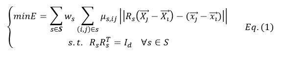
where Xj, xj are the initial and the final position vector of node j respectively, Rs is the rotation matrix of the stencil s, S is the stencil set and ws is a scalar weight per stencil that stresses the importance of some stencils as higher than that of some others’ (e.g. in case of a boundary layer). Regarding μs,ij this is a scalar weight per stencil–edge that accounts for mesh anisotropy. It prevents the distortion of a stencil by favoring/penalizing most the edges that are compressed, handling thus mesh anisotropies. Looking at the quadratic constraint in Eq. (1), it is clear that the problem is non-linear which means that an iterative method is needed to solve it. In the figures that follow, some examples of mesh deformations/shape optimization are shown, in order to show the efficiency of the proposed mesh deformation tool.
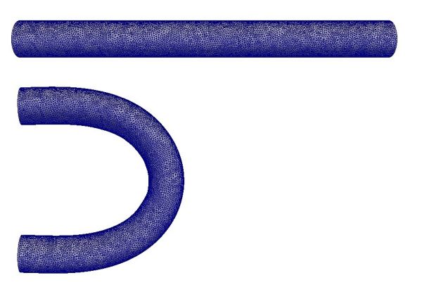
Figure 1: Cylinder under bending deformation. On top, the initial shape is presented whereas the deformed shape is shown on the bottom. The Finite Transformation Rigid Motion Mesh Morpher is used to adapt the volume mesh to the updated boundaries.
CAD-Free Soft Handle Parameterization Tool
In an adjoint-based optimization algorithm, after having computed the sensitivities, the necessary changes should be applied in the shape. The CAD-Free parameterization tool, the Soft Handle Parameterization tool, is responsible for applying the shape changes and the Finite Transformation Rigid Motion Mesh Morpher for adapting the volume mesh to the updated boundaries. The model that describes the Finite Transformation Mesh Morpher and its adaptive Soft Handle CAD-Free parameterization tool, is the following:
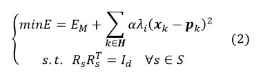
In Eq. (2), EM is the energy to be minimized that corresponds to the Finite Transformation Rigid Motion Mesh Morpher λi is a set of weights, pk the position of the parameter/handle k and H, S the handle/parameter and the stencil set respectively. The first term in the first line of Eq. (2) corresponds to the mesh morpher and the second one to the parameterization tool itself. The parameterization tool cannot work independently from the mesh morpher, thus the shape changes and the adaptation of the volume mesh to the updated boundaries are taking place at the same time. In the figures that follow, the fully-automated workflow is presented.
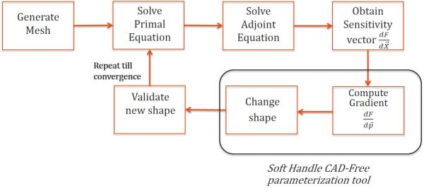
Figure 2: CAD-Free Shape Optimization Workflow.
S-bend optimization
This application is dealing with the S-bend duct, an air duct test case provided by VolksWagen AG. The optimization aims at minimizing J, where J stands for the total pressure losses across the duct.
The baseline mesh consists of 480K nodes and 466K hexahedra. The flow is laminar with inlet velocity u=0,1 m/s (normal to the inlet boundary) and with Reynolds number approximately of Re=400, based on the hydraulic diameter of the inlet. In this case the only part that is allowed to deform is the central curved part. After performing 30 optimization cycles, the total pressure losses are reduced approximately by 23.7% w.r.t. the initial.
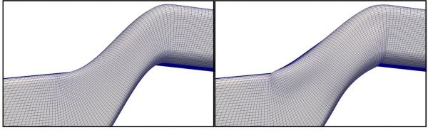
Figure 3: Initial Shape of the duct (left) and optimized one (right).
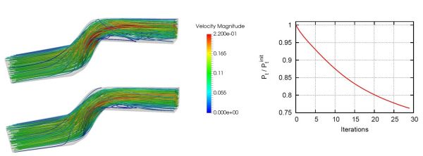
Figure 4: Streamlines in the initial (left up) and in the optimized geometry of the S-bend (left bottom). Convergence history is shown on the right side.
Immersive Visualization
The contribution of ESR 6 regards mainly the immersive visualization of the adjoint results within IC.IDO, ESI’s immersive visualization tool. ESR 6 has integrated these tools into the industrial optimization workflow. The ESR has contributed in the industrial evaluation and benchmarking by providing the capability of providing the outcome of the Adjoint - based Optimization (sensitivity map, adjoint state etc.) inside IC.IDO. Briefly, it is based on the most advanced Virtual Reality technologies and expertise. It facilitates the decision-making process of globally operating interdisciplinary teams, by replacing the need of physical prototypes. IC.IDO, give us the possibility to visualize the sensitivity vector and study it, in order to understand the physics behind the shape that is optimized. The whole fully-automated workflow has been used in industrial shape optimization cases (DrivAer, U-bend, S-bend etc).
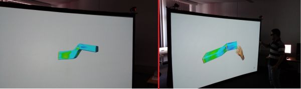
Figure 5: Sensitivity map on the S-bend duct plotted within IC.IDO for the first optimization step.